Multilayer perceptron
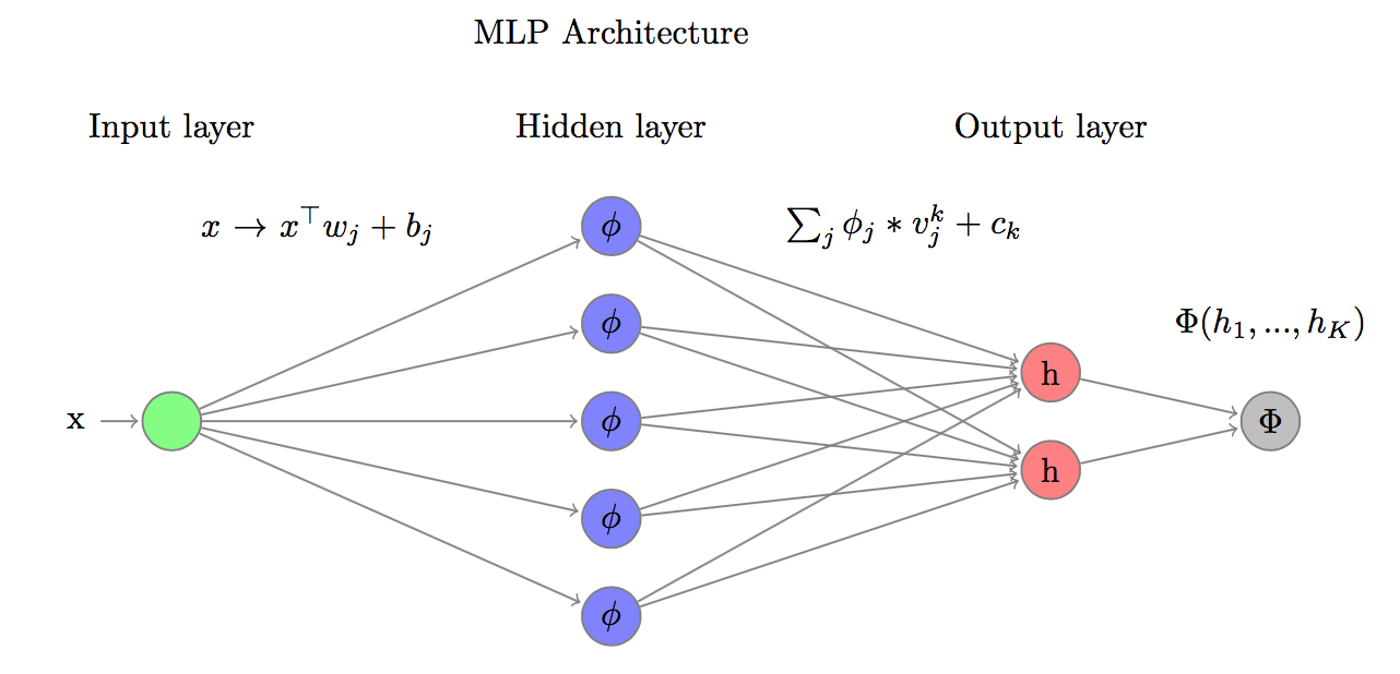
Multilayer perceptron (MLP) is the simplest feed-forward neural network. It mitigates the constraints of original perceptron that was able to learn only linearly separable patterns from the data. It achieves this by introducing at least one hidden layer in order to learn representation of the data that would enable linear separation.

In the first layer MLP apply linear transformations to the data point :
the number of the transformations is the number of hidden nodes in the first hidden layer.
Next it applies non-linear transformation of outputs using so called activation function. Using linear function as a activation function would defeat the purpose of MLP as composition of linear transformations is still linear transformation.
The most often used activation function is so called rectifier:
Finally the outputs of activation function are again combined using linear transformation:
At this point one can either repeat activation step and extend network with next activation layer or apply final transformation of the outputs to fit the algorithm objective. In case of classification problems most often used transformation is softmax function:
which maps real valued vector to a vector of probabilities.
In case of classification problems the most often used loss function is cross-entropy between class label and probability returned by softmax function
which is averaged over all training observations.
Universal Approximation Theorem
According to the theorem first proved by George Cybenko for sigmoid activation function: “feed-forward network with a single hidden layer containing a finite number of neurons (i.e., a multilayer perceptron), can approximate continuous functions on compact subsets of , under mild assumptions on the activation function.”
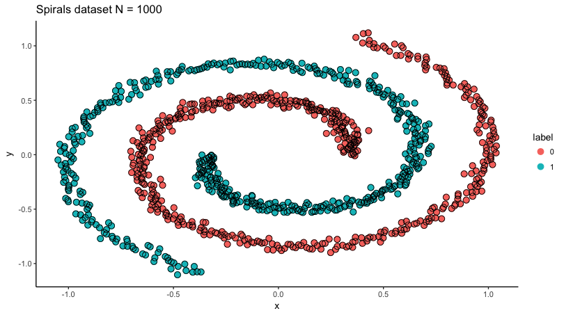
Lets put mlp to the test then. For this purpose I will use sprials dataset from mlbench package.

MXNet
MXNet is an open-source deep learning framework that allows you to define, train, and deploy deep neural networks on a wide array of devices, from cloud infrastructure to mobile devices and it allows to mix symbolic and imperative programming flavors. For example custom loss functions and accuracy measures.
Read more: http://mxnet.io
Network configuration
MXNet package expose so called symbolic API for R users. Its purpose is to create user friendly way of building neural networks abstracting out computational details to the MXNet specialized engine.
Most important symbols:
- mx.symbol.Variable: defines variables (input data, labels, …)
- mx.symbol.FullyConnected: affine transformation of input tensor
- mx.symbol.Activation: places activation function which is applied to all fields of input tensor
- mx.symbol.Output: defines final transformation of data and loss function.
Below is the example of code that configures perceptron with one hidden layer.
  ########### Network configuration ########

  # variables
  act <- mx.symbol.Variable("data")

  # affine transformation
  fc <- mx.symbol.FullyConnected(act, num.hidden = 10)

  # non-linear activation
  act <- mx.symbol.Activation(data = fc, act_type = "relu")

  # affine transformation
  fc <- mx.symbol.FullyConnected(act, num.hidden = 2)

  # softmax output and cross-
  mlp <- mx.symbol.SoftmaxOutput(fc)
Preparing data
  set.seed(2015)

  ############ sprials dataset ############

  s <- sample(x = c("train", "test"),
              size = 1000,
              prob = c(.8,.2),
              replace = TRUE)

  dta <- mlbench.spirals(n = 1000, cycles = 1.2, sd = .03)
  dta <- cbind(dta[["x"]], as.integer(dta[["classes"]]) - 1)
  colnames(dta) <- c("x","y","label")

  ######### train, validate, test ##########

  dta.train <- dta[s == "train",]
  dta.test <- dta[s == "test",]
Network training
Feed-forward networks are trained using iterative gradient descent type of algorithm. Additionally during single forward pass only subset of the data is used called batch. Process is repeated until all training examples are used. This is called an epoch. After every epoch MXNet returns training accuracy:
  ############# basic training #############

  mx.set.seed(2014)
  model <- mx.model.FeedForward.create(
            symbol = mlp,
            X = dta.train[, c("x", "y")],
            y = dta.train[, c("label")],
            num.round = 5,
            array.layout = "rowmajor",
            learning.rate = 1,
            eval.metric = mx.metric.accuracy)
## Start training with 1 devices
## [1] Train-accuracy=0.506510416666667
## [2] Train-accuracy=0.5
## [3] Train-accuracy=0.5
## [4] Train-accuracy=0.5
## [5] Train-accuracy=0.5
Custom call-back
In order to stop process of training when the progress in accuracy is below certain level of tolerance we need to add custom callback to the feed forward procedure. It is called after every epoch to check if algorithm progresses. If not it will terminate optimization procedure and return results.
  ######## custom stopping criterion #######

  mx.callback.train.stop <- function(tol = 1e-3,
                                     mean.n = 1e2,
                                     period = 100,
                                     min.iter = 100
                                     ) {
    function(iteration, nbatch, env, verbose = TRUE) {
      if (nbatch == 0 & !is.null(env$metric)) {
          continue <- TRUE
          acc.train <- env$metric$get(env$train.metric)$value
          if (is.null(env$acc.log)) {
            env$acc.log <- acc.train
          } else {
            if ((abs(acc.train - mean(tail(env$acc.log, mean.n))) < tol &
                abs(acc.train - max(env$acc.log)) < tol &
                iteration > min.iter) |
                acc.train == 1) {
              cat("Training finished with final accuracy: ",
                  round(acc.train * 100, 2), " %\n", sep = "")
              continue <- FALSE
            }
            env$acc.log <- c(env$acc.log, acc.train)
          }
      }
      if (iteration %% period == 0) {
        cat("[", iteration,"]"," training accuracy: ",
            round(acc.train * 100, 2), " %\n", sep = "")
      }
      return(continue)
      }
   }

  ###### training with custom stopping #####

  mx.set.seed(2014)
  model <- mx.model.FeedForward.create(
          symbol = mlp,
          X = dta.train[, c("x", "y")],
          y = dta.train[, c("label")],
          num.round = 2000,
          array.layout = "rowmajor",
          learning.rate = 1,
          epoch.end.callback = mx.callback.train.stop(),
          eval.metric = mx.metric.accuracy,
          verbose = FALSE
          )
## [100] training accuracy: 90.07 %
## [200] training accuracy: 98.88 %
## [300] training accuracy: 99.33 %
## Training finished with final accuracy: 99.44 %
Results
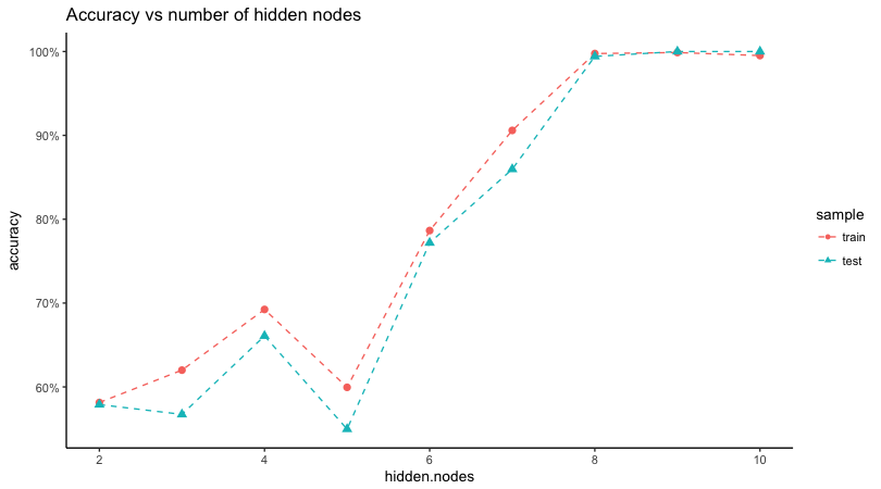
Learning curve

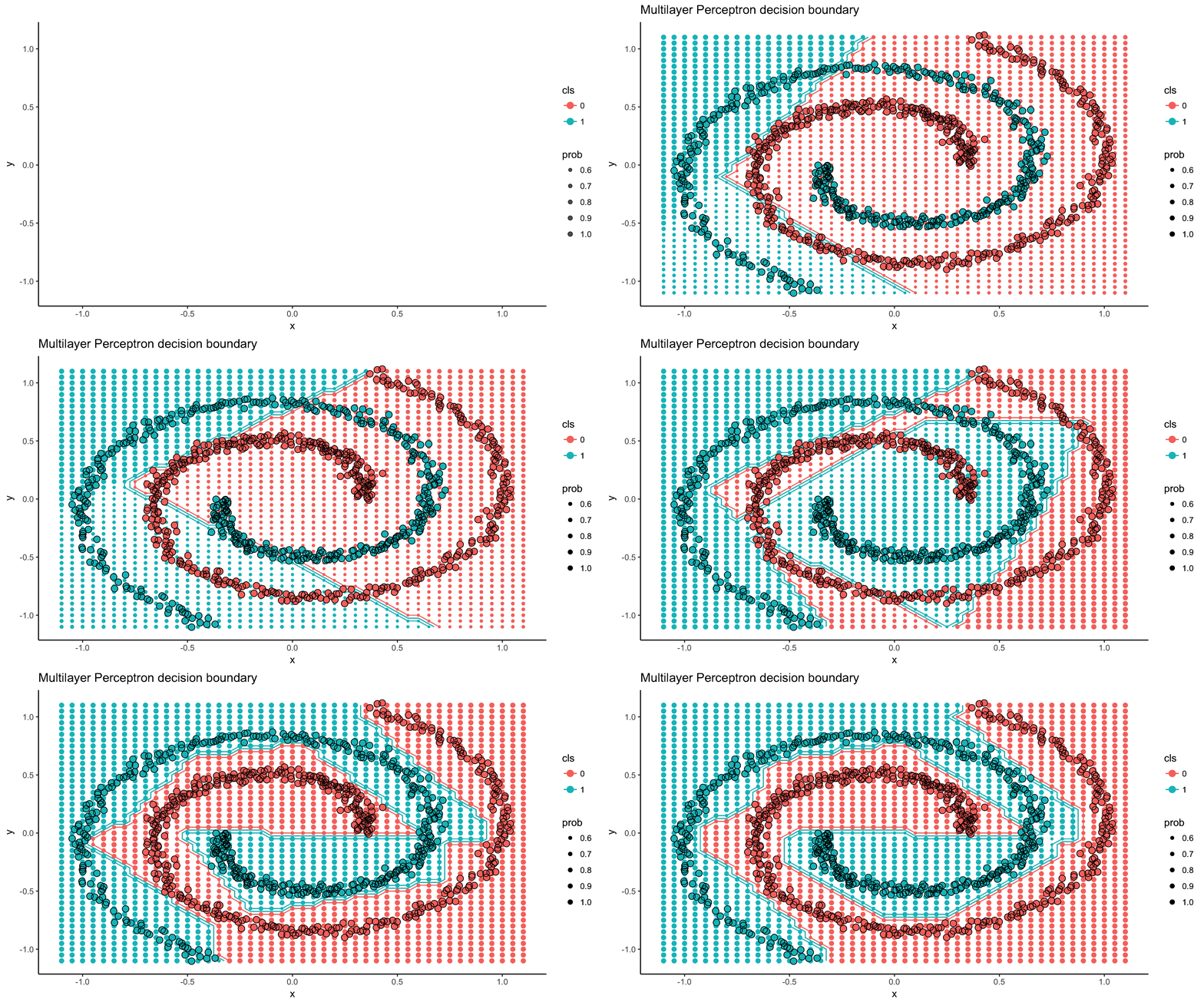
Evolution of decision boundary

Code for this post can be found here: https://github.com/jakubglinka/posts/tree/master/neural_networks_part1